SAMを使った資源量推定

市野川桃子・西嶋翔太

2025-10-20

SAMのインストール

• インストールに必要なパッケージ(devtools)はあらかじめインストールしておいてください

## インストール (最新ブランチはcmsa11→vignetteとかが追加されたcreate_vignette)
#devtools::install_github("ShotaNishijima/frasam@create_vignette") # frasam
## frasyrも使うのでfrasyrもインストールしてください
#devtools::install_github("ichimomo/frasyr@dev")

# ライブラリの呼び出し
library(frasyr)
library(frasam)
# devtools::load_all()
library(tidyverse)
library(patchwork)
# install.packages("lemon")
library(lemon)

SAMを適用するデータセットの作成

VPAを適用するときのデータセットと同じ形式のデータセットが利用できます。 ただし、VPAでは資源量指数が利用できなくても適用できますが、SAMでは資源量指数の利用が必須になります。

データの読み込み

caa   <- read.csv("https://raw.githubusercontent.com/ichimomo/frasyr/dev/data-raw/ex1_caa.csv",  row.names=1)
waa   <- read.csv("https://raw.githubusercontent.com/ichimomo/frasyr/dev/data-raw/ex1_waa.csv",  row.names=1)
maa   <- read.csv("https://raw.githubusercontent.com/ichimomo/frasyr/dev/data-raw/ex1_maa.csv",  row.names=1)
index <- read.csv("https://raw.githubusercontent.com/ichimomo/frasyr/dev/data-raw/ex1_index.csv",  row.names=1)
# create pseudo data for caa
caa   <- caa * exp(rnorm(length(caa), mean=-0.5 * (0.1)^2, sd=0.1))

# Indexがひとつだと例としてあまり適切でないので、適当な加入Indexを作成する
set.seed(2025)
rec_idx <- seq(1,0.25,length=10)*exp(rnorm(10,0,0.2))
index[2,] <- rec_idx

dat <- data.handler(caa=caa, waa=waa, maa=maa, M=0.5, index=index)

# まずはsamのhelpファイルを閲覧してどんなオプションがあるか把握しましょう
#help(sam)

# SAMを使う準備 (samのオプションtmb.run=TRUEでも良いかもだけど、今はうまく動かないみたい？)
use_sam_tmb(TmbFile="sam2",overwrite=FALSE) #compile and activate
#> [1] TRUE

# samの実施
# (*)の部分が設定ポイント
res_sam <- sam(dat,
               last.catch.zero = FALSE,
               cpp.file.name = "sam2",
               tmb.run = FALSE, # TRUEにするとtmbをコンパイルしてロードする。最初の１回だけTRUEにするのが良い？sam2だと動かない
               rec.age = 0,
               plus.group = TRUE,
               alpha = 1, # 最高年齢と最高年齢-1歳のFが同じと仮定（VPAと同じ仮定)
               est.method = "ml",
               # 資源量指数に関わる設定。資源量指数の数だけベクトルで与える。
               abund = c("SSB", "N"),
               min.age = c(0, 0),
               max.age = c(6, 0),
               b.est = FALSE, # b推定の有無(*)
               b.fix = NA,
               # 分散に関わる設定。どの分散を同じとするか。年齢の数だけ与える (*)
               varC =  c(0,0,0,0,0,0,0),　#とりあえずすべての年齢で共通
               varN = c(0,1,1,1,1,1,1),　#0歳と1歳魚以上で分ける
               varF = c(0,0,0,0,0,0,0),   #とりあえずすべての年齢で共通
               # 1歳魚以上のlog(N)のプロセス誤差を小さい値で固定(分散の値なので、この場合SD=0.01に相当)
               varN.fix = c(NA, 1e-4),
               # 再生産関係推定に関わる設定 (*)
               SR = "BH",
               AR = 0,
               # Fの多変量Random walkの非対角成分の相関係数のタイプ。１ならすべての年齢間で相関係数1, 0なら完全にランダム, 2は任意の年齢間で共通のrhoを推定、3は年齢i,jの相関を\eqn{\rho^|i-j|}で推定 (*)
               rho.mode = 0,
               # 初期値の設定
               q.init = NULL,
               sdFsta.init = NULL,
               sdLogN.init = c(0.2, 0.2),
               sdLogObs.init = NULL,
               rho.init = NULL,
               a.init = NULL,
               b.init = NULL,
               # その他
               # ref.year = 1:5, # 重要そうだけど使われていない
               bias.correct = TRUE,
               bias.correct.sd = FALSE,
               get.random.vcov = FALSE,
               silent = TRUE,
               remove.Fprocess.year = NULL,
               RW.Forder = 0,
               map = NULL, # map (パラメータの推定の有無を個別に調整する) を入れる
               map.add = NULL, # mapを追加する
               p0.list = NULL,
               scale = 1000,
               scale_number = 1000,
               gamma = 10,
               sel.def = "max",
               use.index = NULL,
               upper = NULL,
               lower = NULL,
               index.key = NULL,
               index.b.key = NULL,
               lambda = 0,
               add_random = NULL,
               tmbdata = NULL,
               sep_omicron = TRUE,
               catch_prop = NULL,
               no_est = FALSE,
               getJointPrecision = FALSE,
               loopnum = 2
)

## 推定結果の確認: opt=推定パラメータや目的関数、収束の有無
## - $convergenceが0なら収束
res_sam$opt
#> $par
#>         logQ         logQ logSdLogFsta    logSdLogN  logSdLogObs  logSdLogObs 
#>     9.589461    -7.157883    -1.872021    -1.633707    -2.754415    -1.360896 
#>  logSdLogObs     rec_loga     rec_logb 
#>    -1.611545     2.346322   -18.267778 
#> 
#> $objective
#> [1] -5.25335
#> 
#> $convergence
#> [1] 0
#> 
#> $iterations
#> [1] 66
#> 
#> $evaluations
#> function gradient 
#>       95       67 
#> 
#> $message
#> [1] "relative convergence (4)"

## 推定結果の確認: rep=推定パラメータとSE
## - 推定値(Estimate)に対してStd.Errorが異常に大きくないか
## - Maximum gradient componentが十分小さい値か（1e-3以下なら十分OK、多数のパラメータを推定する難しいモデルなら上限0.1以下くらいでも？)
res_sam$rep
#> sdreport(.) result
#>                Estimate   Std. Error
#> logQ           9.589461 9.073807e-02
#> logQ          -7.157883 7.018642e-02
#> logSdLogFsta  -1.872021 1.589935e-01
#> logSdLogN     -1.633707 2.634245e-01
#> logSdLogObs   -2.754415 4.934159e-01
#> logSdLogObs   -1.360896 2.360906e-01
#> logSdLogObs   -1.611545 2.371708e-01
#> rec_loga       2.346322 7.373170e-02
#> rec_logb     -18.267778 1.389361e+04
#> Maximum gradient component: 1.587814e-05

## 推定結果の確認: AIC（単独ではあまり意味がない。モデルを比較するときに）
res_sam$aic
#> [1] 7.493301

## 推定結果の確認: 分散パラメータのsigma。ノーマルスケールで、大きさを確認。
## - すごく小さい値で推定されている場合には推定の意味がないので推定しないなどする
## - どのsigmaを共通にするか？を決める
res_sam[c("sigma","sigma.logC","sigma.logFsta","sigma.logN")]
#> $sigma
#> [1] 0.2564308 0.1995790
#> 
#> $sigma.logC
#> [1] 0.06364625 0.06364625 0.06364625 0.06364625 0.06364625 0.06364625 0.06364625
#> 
#> $sigma.logFsta
#> [1] 0.1538125 0.1538125 0.1538125 0.1538125 0.1538125 0.1538125 0.1538125
#> 
#> $sigma.logN
#> [1] 0.1952047 0.0100000 0.0100000 0.0100000 0.0100000 0.0100000 0.0100000

## 固定効果の確認・出力
fixef = out_par(res_sam,filename="FEpar")
knitr::kable(fixef)

FE	MLE	SE	Gradient	Unlinked value
logQ	9.589461	9.073810e-02	5.80e-06	1.460999e+04
logQ	-7.157883	7.018640e-02	1.59e-05	7.787000e-04
logSdLogFsta	-1.872021	1.589935e-01	1.22e-05	1.538125e-01
logSdLogN	-1.633707	2.634245e-01	4.20e-06	1.952047e-01
logSdLogObs	-2.754415	4.934159e-01	2.80e-06	6.364630e-02
logSdLogObs	-1.360896	2.360906e-01	-5.00e-06	2.564308e-01
logSdLogObs	-1.611545	2.371708e-01	2.60e-06	1.995790e-01
rec_loga	2.346322	7.373170e-02	1.03e-05	1.044708e+01
rec_logb	-18.267778	1.389361e+04	0.00e+00	0.000000e+00

## 結果の出力
out_sam(res_sam, filename="sam")

## VPAもやってみる
res_vpa <- vpa(dat,fc.year=1998:2000,tf.year = 1998:1999,
               term.F="max",stat.tf="mean",Pope=TRUE,tune=TRUE,p.init=0.5, abund=c("SSB","N"), min.age=c(0,0), max.age=c(6,0), sel.update=TRUE)

## VPAとSAMのモデルの比較
gg_graph1 <- plot_vpa(list(VPA=res_vpa, SAM=res_sam))
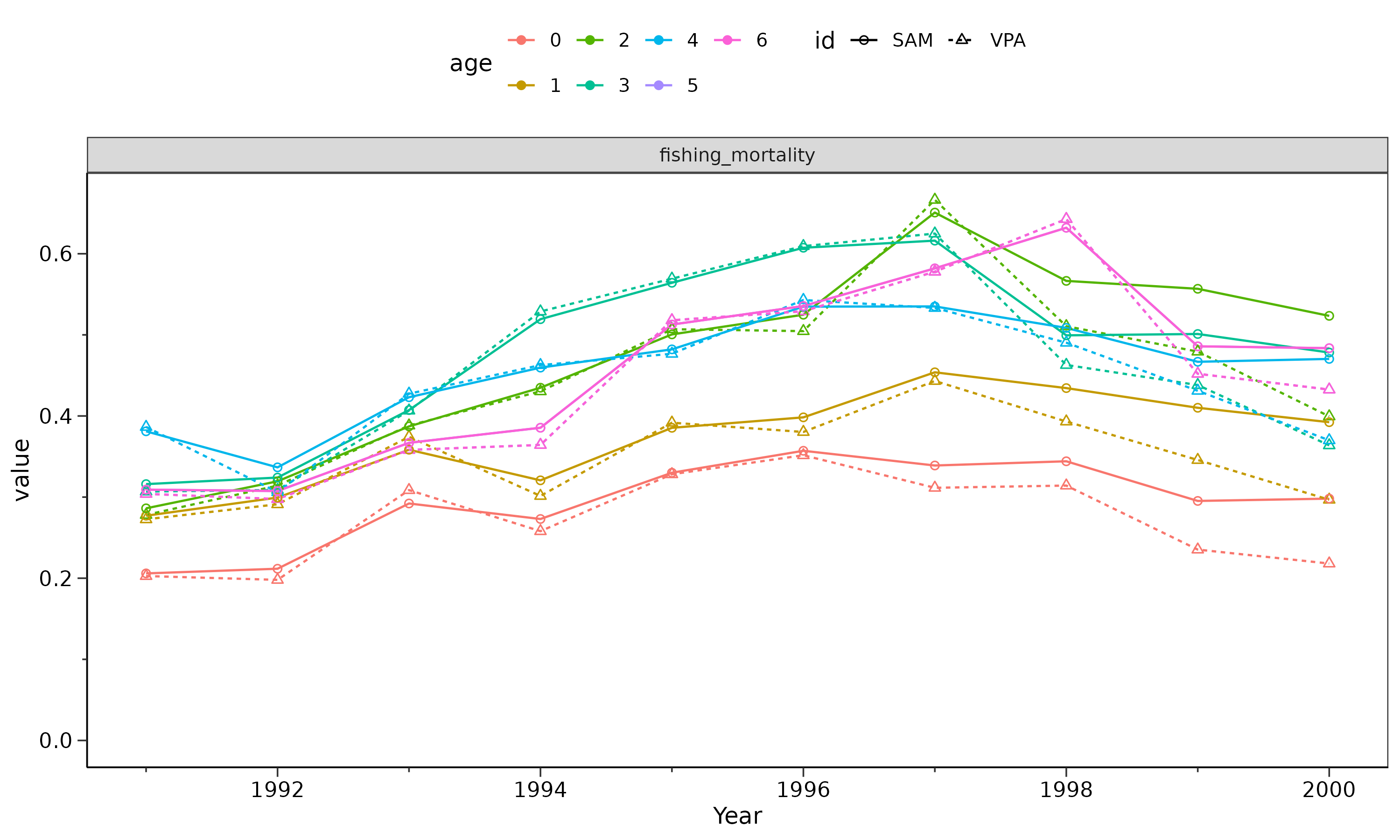
gg_graph2 <- plot_vpa(list(VPA=res_vpa, SAM=res_sam), what.plot=c("fishing_mortality"))

print(gg_graph1)
print(gg_graph2)


## 設定を少し変えてもう一度実行する場合
sam_input <- res_sam$input # samに渡した引数のリスト
sam_input$rho.mode <- 1 # 引数の一部を変える（たとえば、Fの相関を1にする→今は選択率一定)
res_sam2 <- do.call(sam, sam_input) # do.callで再度計算
res_sam2$opt #収束している
#> $par
#>         logQ         logQ logSdLogFsta    logSdLogN  logSdLogObs  logSdLogObs 
#>     9.567369    -7.182519    -2.088952    -1.693182    -2.254609    -1.415567 
#>  logSdLogObs     rec_loga     rec_logb 
#>    -1.671908     2.347437   -20.512563 
#> 
#> $objective
#> [1] -18.62319
#> 
#> $convergence
#> [1] 0
#> 
#> $iterations
#> [1] 85
#> 
#> $evaluations
#> function gradient 
#>      112       86 
#> 
#> $message
#> [1] "relative convergence (4)"
res_sam2$rep #sdreportの結果
#> sdreport(.) result
#>                Estimate   Std. Error
#> logQ           9.567369 9.020410e-02
#> logQ          -7.182519 7.350979e-02
#> logSdLogFsta  -2.088952 2.715267e-01
#> logSdLogN     -1.693182 2.618395e-01
#> logSdLogObs   -2.254609 1.126745e-01
#> logSdLogObs   -1.415567 2.355007e-01
#> logSdLogObs   -1.671908 2.441719e-01
#> rec_loga       2.347437 6.843250e-02
#> rec_logb     -20.512563 4.122388e+04
#> Maximum gradient component: 5.003338e-05
res_sam2$rep$pdHess #Hessianが正定値を持つかどうか（持たない場合SEが計算できない）
#> [1] TRUE

## 2つのモデルのAICの比較
## - 選択率一定モデルのほうがAICが小さい（＝より予測力が高い）
c(res_sam$aic, res_sam2$aic)
#> [1]   7.493301 -19.246374

c(res_sam$rho, res_sam2$rho) #Fの相関係数
#> [1] 0 1

sam_input$SR <- "RW" #加入をRWに変更
res_sam3 <- do.call(sam,sam_input)
res_sam3$opt　
#> $par
#>         logQ         logQ logSdLogFsta    logSdLogN  logSdLogObs  logSdLogObs 
#>     9.557986    -7.189545    -2.080289    -1.113911    -2.250367    -1.430761 
#>  logSdLogObs 
#>    -1.665477 
#> 
#> $objective
#> [1] -13.58094
#> 
#> $convergence
#> [1] 0
#> 
#> $iterations
#> [1] 48
#> 
#> $evaluations
#> function gradient 
#>       66       48 
#> 
#> $message
#> [1] "both X-convergence and relative convergence (5)"
res_sam3$rep
#> sdreport(.) result
#>               Estimate Std. Error
#> logQ          9.557986 0.09000536
#> logQ         -7.189545 0.07421993
#> logSdLogFsta -2.080289 0.27342451
#> logSdLogN    -1.113911 0.25226177
#> logSdLogObs  -2.250367 0.11344229
#> logSdLogObs  -1.430761 0.23392965
#> logSdLogObs  -1.665477 0.24375664
#> Maximum gradient component: 2.588278e-06
res_sam3$rep$pdHess
#> [1] TRUE

c(res_sam$aic, res_sam2$aic, res_sam3$aic)
#> [1]   7.493301 -19.246374 -13.161880


## SAMだけの比較 (fishing_mortalityはFの平均？)
## - 信頼区間付きバージョン
## - VPAの結果も並列で示せるが、その場合vpa関数の実行にはTMB=TRUEオプションをつける必要あり
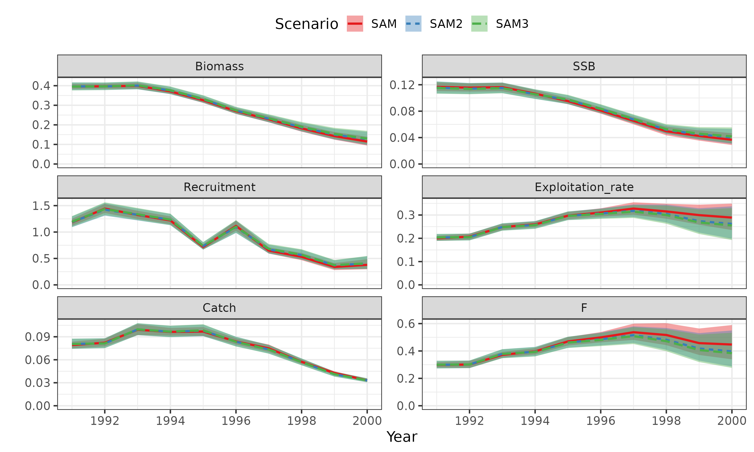
plot_samvpa(list(SAM=res_sam, SAM2=res_sam2,SAM3=res_sam3),
            what.plot = c("biomass","SSB","Recruitment","U","catch","fishing_mortality"))

## 結果の出力
## - 境さん関数(make_assess_result)
## - out.vpa(out_samなら動く)、convert_vpa_tibbleも動くようにしたい
res_samdata <- make_assess_result(res_sam)

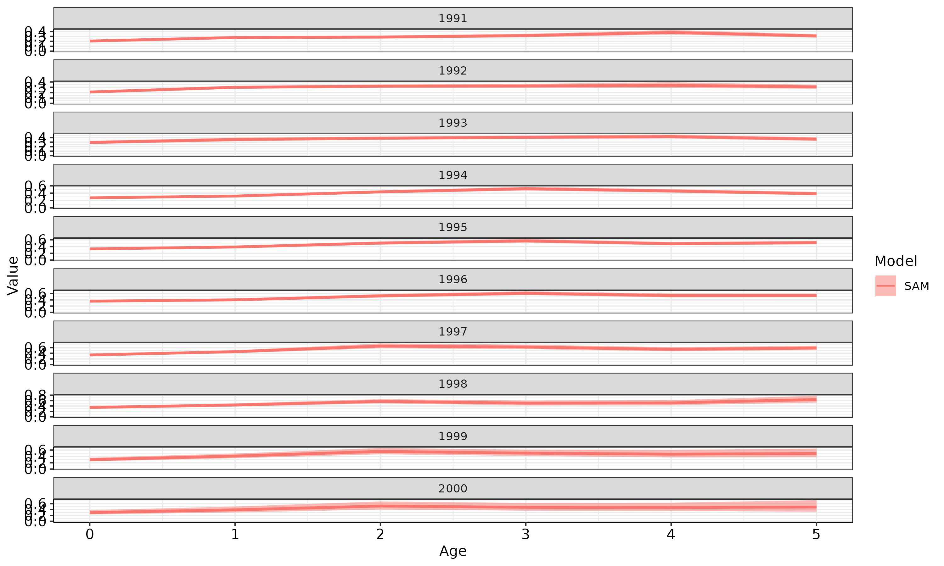
## F at age by year (境さんコード、関数化必要？時系列が長い場合への対応が必要)
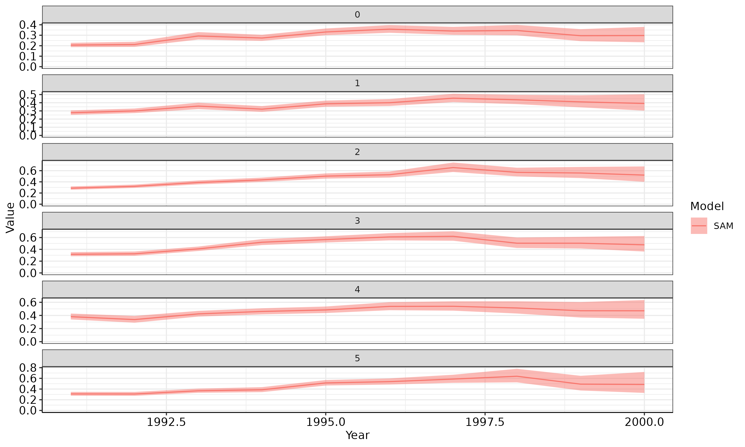
(gg <- res_samdata %>% dplyr::filter(stat=="faa") %>%
    ggplot() +
    geom_ribbon(aes(x=Age, ymax=upper, ymin=lower, group=Model, fill=Model), alpha=0.5) +
    geom_line(aes(x=Age, y=Value, colour=Model, group=Model, size=Model), linetype=1) +
    facet_wrap(.~Year, scales = "free_y", nrow=10, ncol=2, dir="v") +
    scale_y_continuous(limits = c(0, NA)) +
    scale_fill_manual("Model", values = c("#F8766D", "black")) +
    scale_colour_manual("Model", values = c("#F8766D", "black")) +
    scale_size_manual("Model", values = c(1, 0.5), guide = "none") +
    theme_bw() + 
    # labs(title="FAA", x=xlab, y=ylab) +
    theme(axis.text.x = element_text(size = 11, color = "black"),
          axis.text.y = element_text(size = 11, color = "black"),
          axis.line.x = element_line(linewidth = 0.3528), axis.line.y = element_line(linewidth = 0.3528),
          axis.minor.ticks.length = rel(0.5)))

## F at age by year
(gg <- res_samdata %>% dplyr::filter(stat=="faa") %>%
    mutate(Age=factor(Age)) %>%
    ggplot() +
    geom_ribbon(aes(x=Year, ymax=upper, ymin=lower, group=Model, fill=Model), alpha=0.5) +
    geom_line(aes(x=Year, y=Value, colour=Model, group=Model), linetype=1) +
    facet_wrap(.~Age, scales = "free_y", nrow=10, ncol=2, dir="v") +
    scale_y_continuous(limits = c(0, NA)) +
    #  scale_fill_manual("Model", values = c("#F8766D", "black")) +
    #  scale_colour_manual("Model", values = c("#F8766D", "black")) +
    #  scale_size_manual("Model", values = c(1, 0.5), guide = "none") +
    theme_bw() + 
    # labs(title="FAA", x=xlab, y=ylab) +
    theme(axis.text.x = element_text(size = 11, color = "black"),
          axis.text.y = element_text(size = 11, color = "black"),
          axis.line.x = element_line(linewidth = 0.3528), axis.line.y = element_line(linewidth = 0.3528),
          axis.minor.ticks.length = rel(0.5)))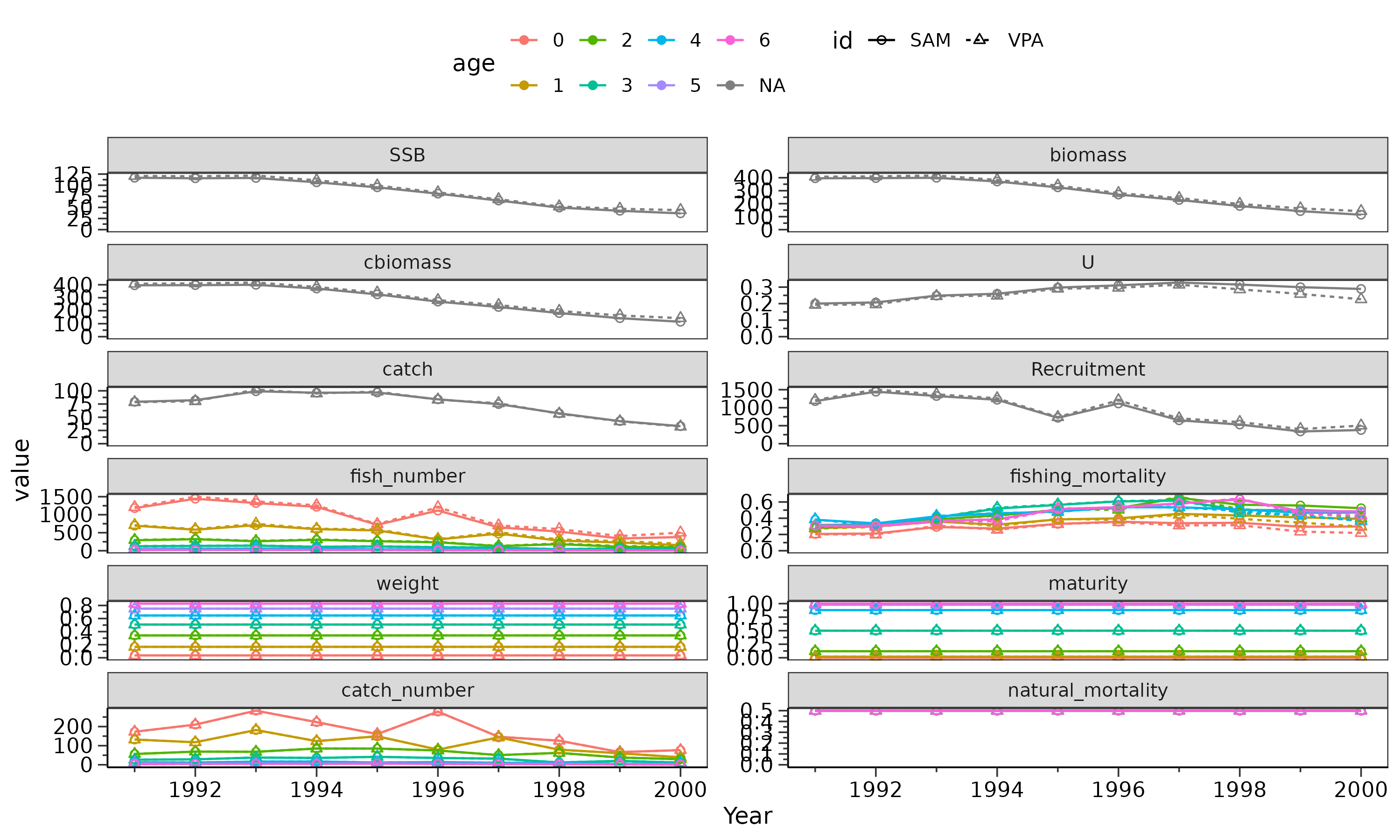

モデル選択

• rho.mode 0, 1, 2, 3のどれか？
• 再生産関係の関数と自己相関
• どの要素でsigmaを推定値し、どの年齢間でsigmaを共通にするか?
  • いろいろ試してAICの小さいものを選ぶ。（最新のcAICというものもあるようだが、未実装）

## varF(Fのプロセス誤差)とvarC（CAAの観測誤差）をどの年齢間で分けるかをstepAICで検討する

# いまは1歳魚以上のvarNを固定しているが、それも検討することも可能
# 検討する変数(VarF, VarC)を境界を入れる年齢Xについてのデータを生成(varとXを列名に使用)
# ここでは収束しやすさからRWの場合を使用する（BHを使うとlog(b)->-InfになりSEが発散する
grid = expand.grid(var=c("varF","varC"),X=1:6) %>%
  filter(!(var == "varF" & X == 6)) #5-6歳のFは同じと仮定しているので6歳は不要なので除いておく

res_select <- select_sigma_grid(
  res_sam2, grid=grid, check_converge = TRUE, SEmax=Inf) # convergeしてるもののうちAIC最少を選ぶように変更
## Best modelの結果チェック
# FAAの誤差が0歳と1歳以上で分かれる
cbind(
  "Age" = 0:6,
  "SD_caa" = res_select$bestres$sigma.logC,
  "SD_faa" = res_select$bestres$sigma.logF,
  "SD_naa" = res_select$bestres$sigma.logN
) %>% knitr::kable()

Age	SD_caa	SD_faa	SD_naa
0	0.1049146	0.1238168	0.1839333
1	0.1049146	0.1238168	0.0100000
2	0.1049146	0.1238168	0.0100000
3	0.1049146	0.1238168	0.0100000
4	0.1049146	0.1238168	0.0100000
5	0.1049146	0.1238168	0.0100000
6	0.1049146	0.1238168	0.0100000

res_best <- res_select$bestres #AIC最少をベストモデルとする

再生産関係のプロット

## 単純なプロット
plot_SR_simple(res_best)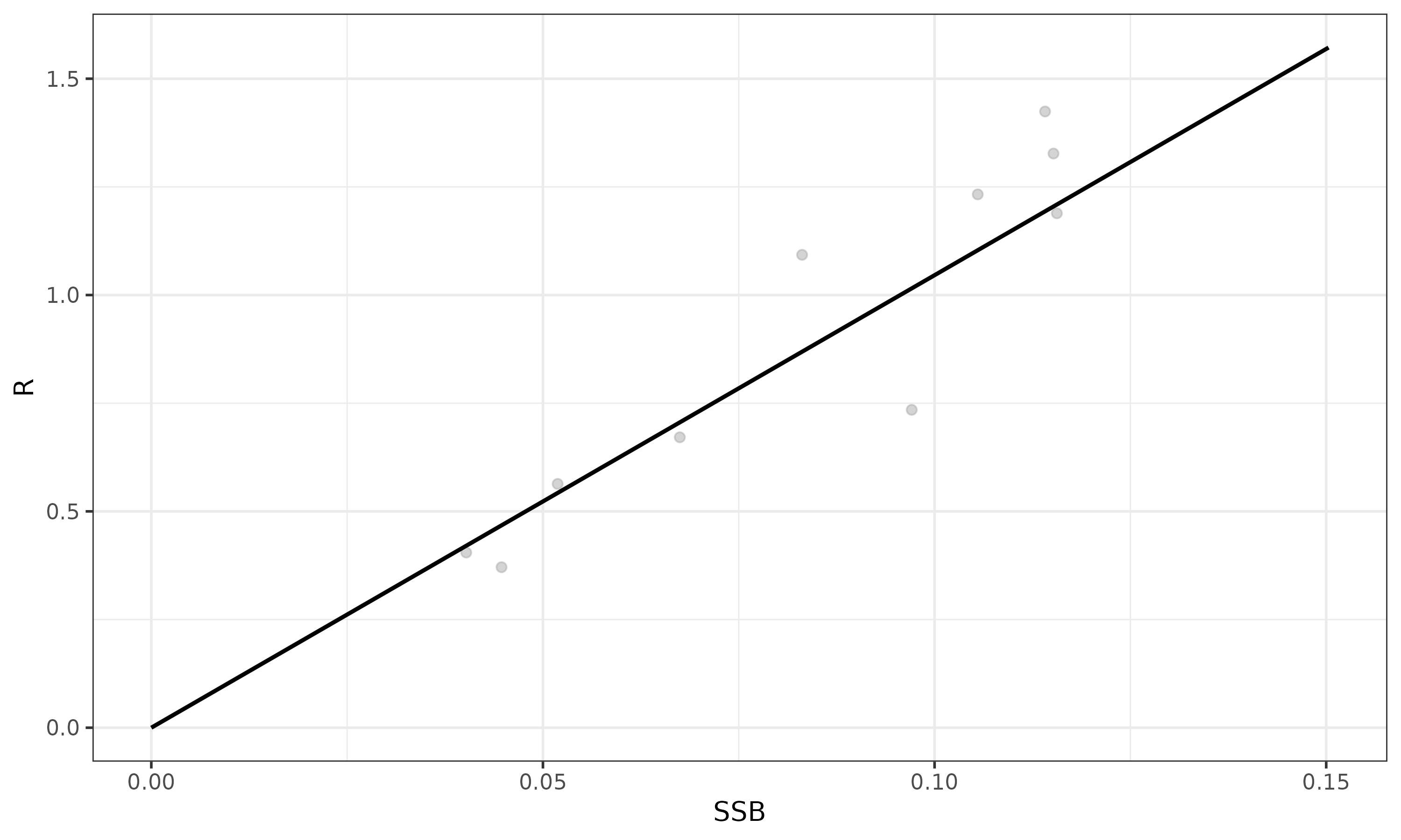

## SAMの結果からfraysrで使える再生産関係のオブジェクトを作成するとfrasyrの関数が使える
SR_sam0 <- res_best %>% make_SRres
biopar <- derive_biopar(res_best, derive_year=1998:2000)
## steepness, R0, B0, 決定論的なMSY管理基準値の計算
steepness_sam <- calc_steepness(SR="BH", rec_pars=SR_sam0$pars,M=biopar$M, waa=biopar$waa, maa=biopar$maa, faa=biopar$faa)
## 再生産関係に依存しない管理基準値の計算(frasyr::ref.F)
# FcurrentとPope=FALSEを明示的に引数に含める必要がある
Fcurrent <- rowMeans(res_best$faa[,as.character(1998:2000)])
refF_res <- ref.F(res_best,Fcurrent=Fcurrent,Pope=FALSE)

refF_res$summary
#>            Fcurrent Fmed Flow Fhigh      Fmax      F0.1 Fmean FpSPR.10.SPR
#> max       0.4871229   NA   NA    NA 0.5623093 0.3412731    NA    0.6748425
#> mean      0.4322984  NaN  NaN   NaN 0.4990227 0.3028636   NaN    0.5988906
#> Fref/Fcur 1.0000000   NA   NA    NA 1.1543478 0.7005893    NA    1.3853640
#>           FpSPR.20.SPR FpSPR.30.SPR FpSPR.40.SPR FpSPR.50.SPR FpSPR.60.SPR
#> max          0.4387275    0.3144842    0.2320948    0.1713765    0.1237870
#> mean         0.3893498    0.2790898    0.2059731    0.1520884    0.1098550
#> Fref/Fcur    0.9006505    0.6455952    0.4764605    0.3518136    0.2541186
#>           FpSPR.70.SPR FpSPR.80.SPR FpSPR.90.SPR
#> max         0.08495827   0.05235453   0.02438887
#> mean        0.07539642   0.04646215   0.02164396
#> Fref/Fcur   0.17440828   0.10747704   0.05006718

モデル診断

残差プロット

## 資源量指数 (frasyrのplot_residual_vpaと統合してもよい？）
## - これは通常のresidual
resid_sam <- index_plot(res_best); wrap_plots(resid_sam)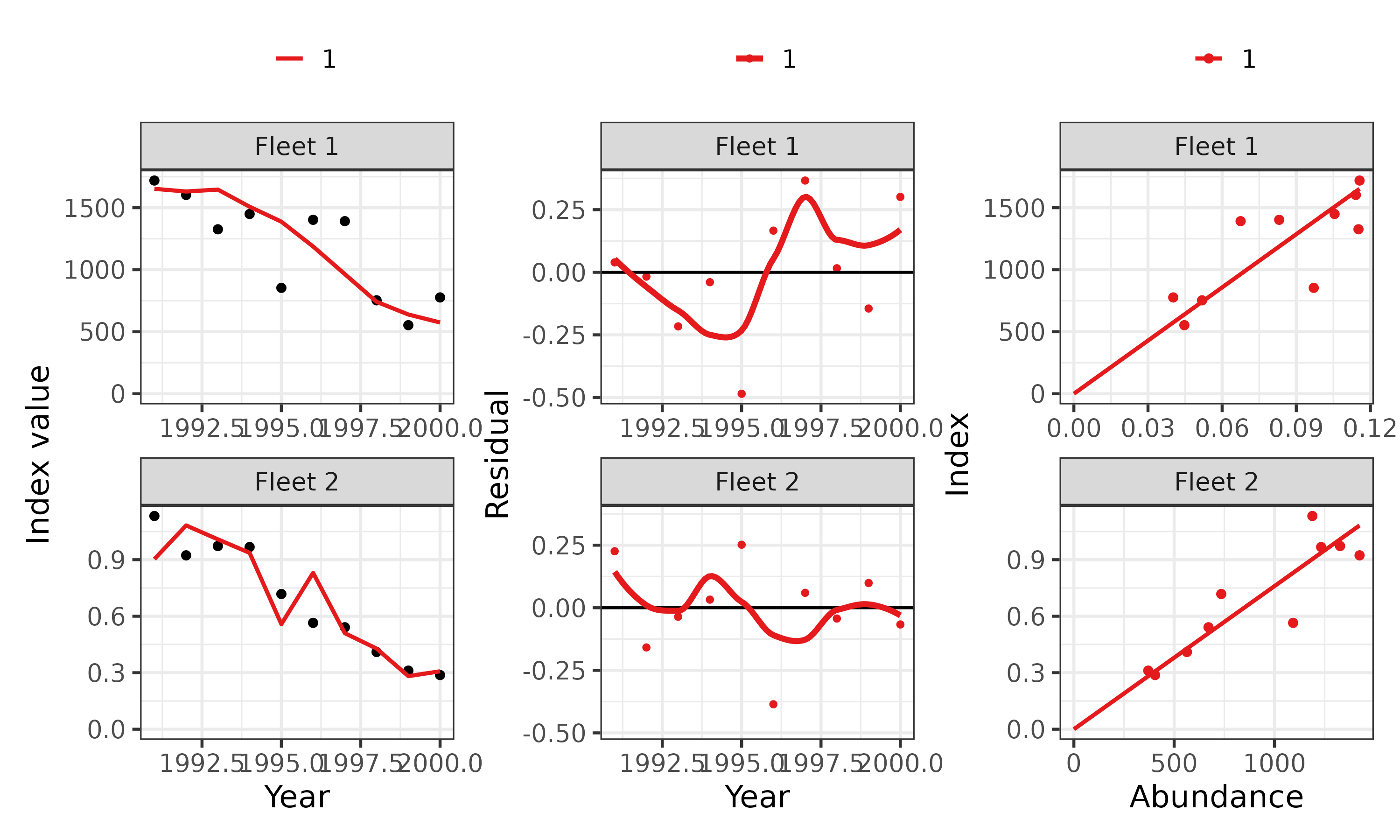

## - OSAは？ => 後で紹介する予定

## catch at age
## -
caa_resid <- caa_plot(res_best); wrap_plots(caa_resid)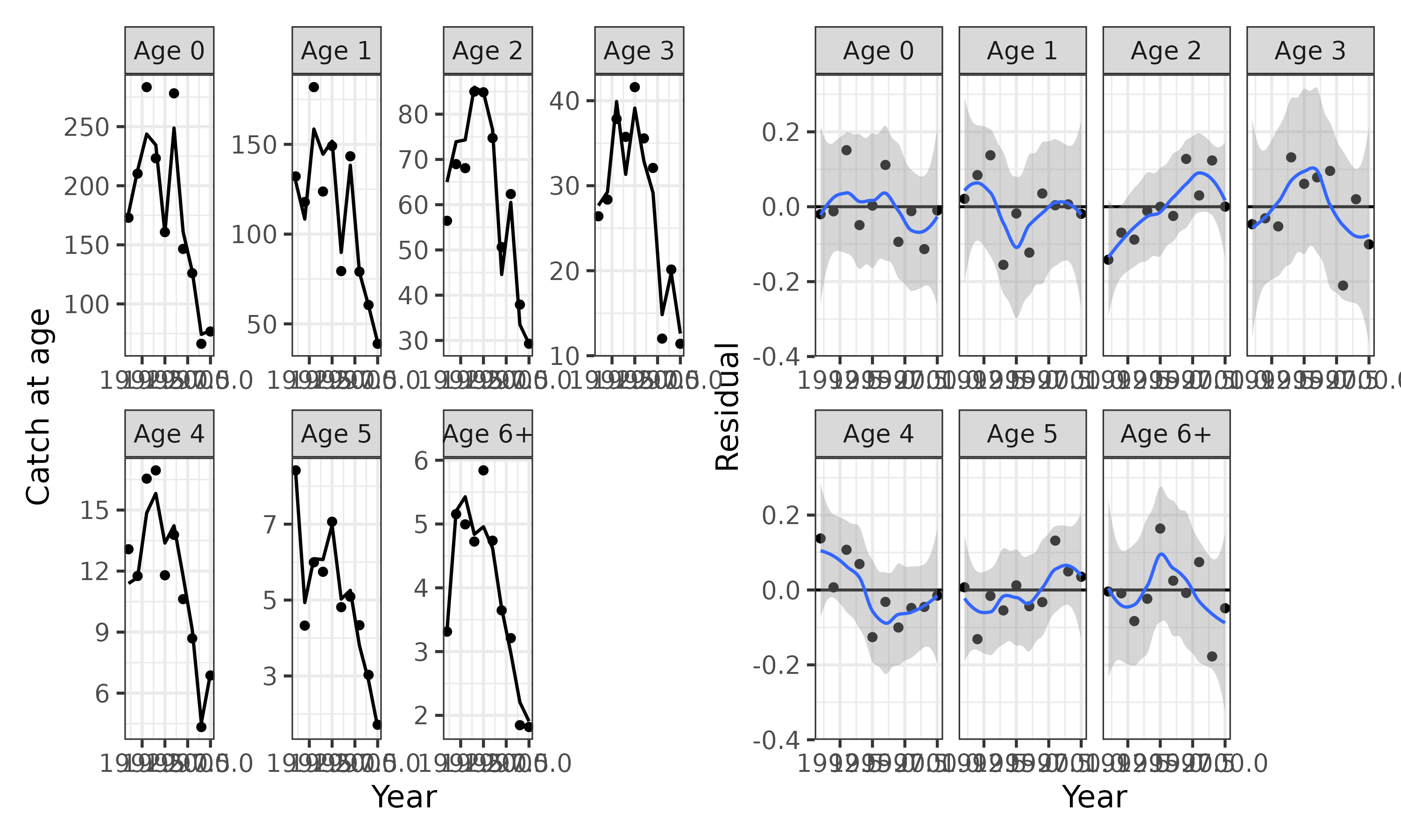

## total catch weight の比較も必要かも
# 今関数はない

# catch at age (sakai ver.)

caa_obs0 <- dat$caa %>% rownames_to_column(var="Age") %>% pivot_longer(cols=-Age, names_to="Year", values_to="Value") %>% mutate(Data="Observation")
caa_est0 <- res_best$caa %>% as.data.frame %>% rownames_to_column(var="Age") %>% pivot_longer(cols=-Age, names_to="Year", values_to="Value") %>% mutate(Data="Estimation")
caa_obs_est <- bind_rows(caa_obs0, caa_est0)

xlab <- "年齢"
ylab <- "漁獲尾数（百万尾）"
scale <- 1000
g1 <- ggplot() +
  geom_bar(data=caa_obs0, stat="identity", aes(x=Age, y=Value/scale), col="black", fill="#FFFFB3") +
  geom_line(data=caa_est0, aes(x=Age, y=Value/scale, group=Data), col="#F8766D", linewidth=1.5) +
  facet_wrap(~Year, scales = "free_y", nrow=10, dir="v") +
  ylim(c(0, NA)) + scale_x_discrete(limit = c("0", "1", "2", "3", "4", "5", "6", "7", "8+")) +
  theme_bw() + labs(title="CAAプロット(棒グラフ：観測値, 折れ線：推定値)", x=xlab, y=ylab) +
  theme(axis.text.x = element_text(size = 11, color = "black"),
        axis.text.y = element_text(size = 11, color = "black"),
        axis.line.x = element_line(linewidth = 0.3528), axis.line.y = element_line(linewidth = 0.3528),
        axis.minor.ticks.length = rel(0.5), legend.position = "none")

レトロスペクティブ解析

• という関数で実行可能
• Retrospective forecastingも同時に実行可能でプロットもできる

retro_res = retro_sam(res_best,n=5) #nは年数

(g_retro = retro_plot(res_best,retro_res,start_year=1991,mohn_position="bottomleft"))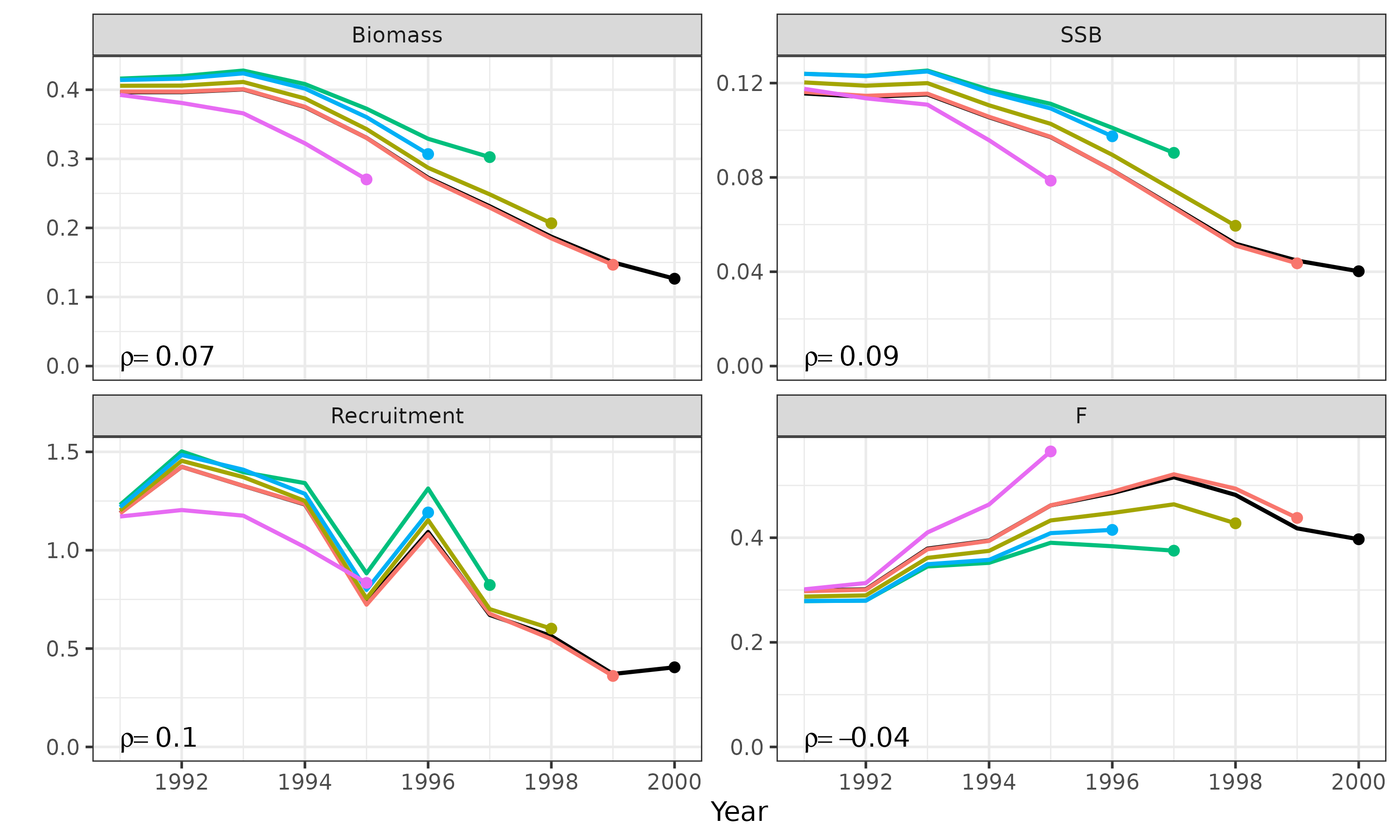

# retrospective forecastingもできる
(g_retro2 = retro_plot(res_best,retro_res,start_year=1991,mohn_position="bottomleft", forecast=TRUE))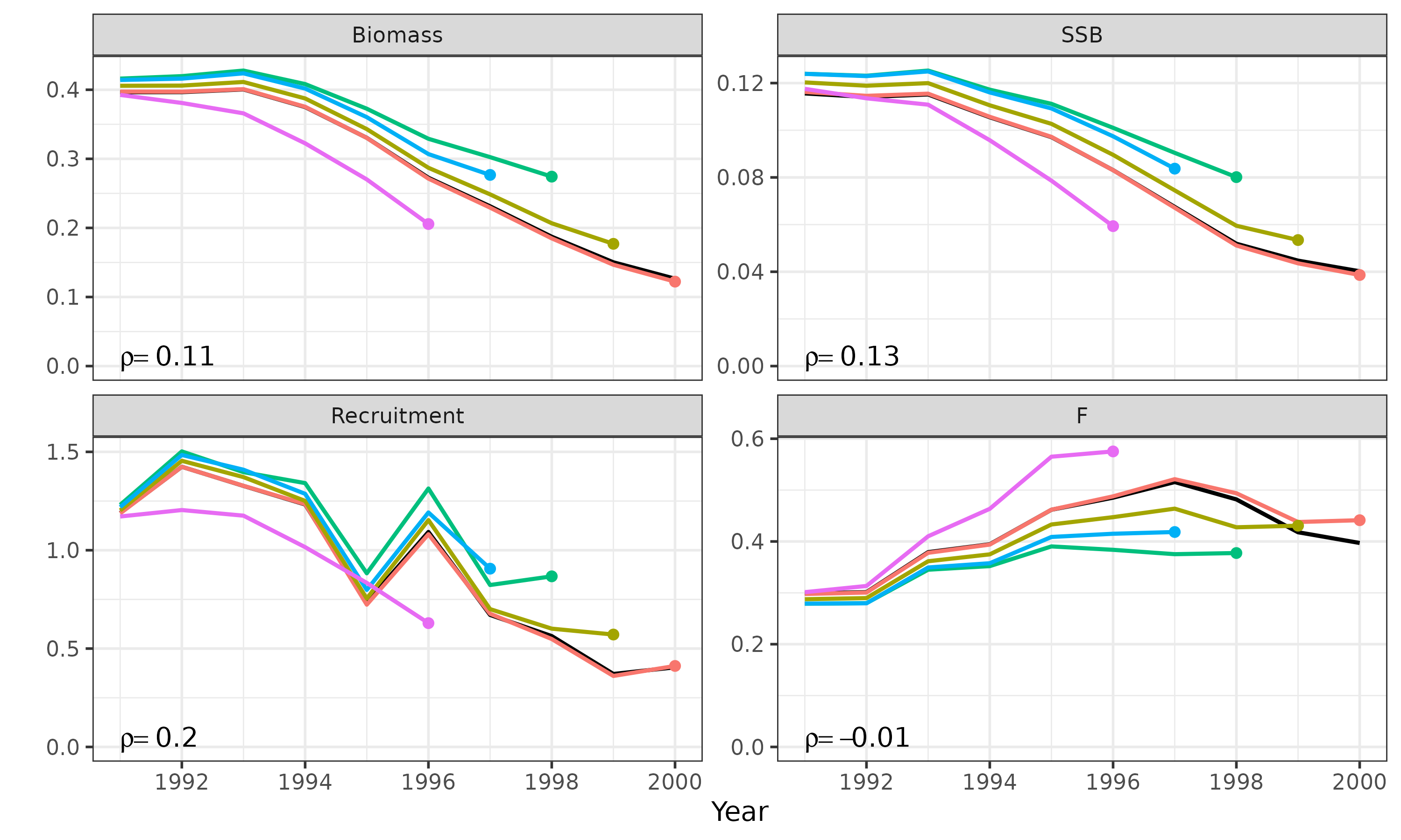

Leave-one-out index analysis

• Indexを一つずつの除いて、推定値の頑健性、影響力のあるIndexを明らかにする（ジャックナイフ解析？）
• という関数を使って実行する

loo_res <- do_loo_index(res_best)
reslist <- list()
for ( j in 0:length(loo_res)) {
    if(j==0) {
      reslist[[j+1]] <- res_best
    } else {
      reslist[[j+1]] <- loo_res[[j]]
    }
}
(g_loo <- plot_samvpa(reslist,CI=0,
                    scenario_name = c("full",as.character(-1:-2))))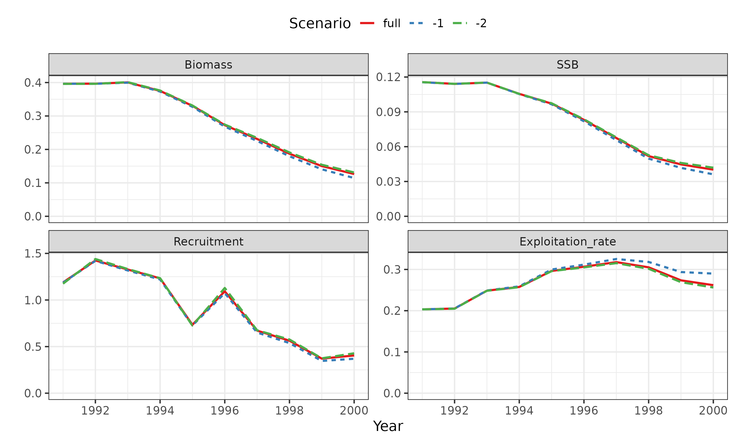

One-Step-Ahead (OSA) residuals

• SAMはランダム効果モデルなので、ハイパーパラメータとランダム効果の推定でデータを二重に使っていることになる
• ランダム効果でデータに対して過度に合わせることも可能であり（過剰適合）、通常の残差を診断に使うのは適切ではないと考えられている
• また、時系列解析なので残差は独立ではないので、独立とみなした診断（QQ plotなど）は不適
• あるサンプルを除いた時の予測値（One Step Ahead (OSA) prediction）とデータとの残差 (OSA residuals) を診断に使うのがより適切らしい
• を使って行うが、SAM用の関数を用意してある

osa.simple <- do_osa_resid(res_best)
#> [1] 90
#> [1] 89
#> [1] 88
#> [1] 87
#> [1] 86
#> [1] 85
#> [1] 84
#> [1] 83
#> [1] 82
#> [1] 81
#> [1] 80
#> [1] 79
#> [1] 78
#> [1] 77
#> [1] 76
#> [1] 75
#> [1] 74
#> [1] 73
#> [1] 72
#> [1] 71
#> [1] 70
#> [1] 69
#> [1] 68
#> [1] 67
#> [1] 66
#> [1] 65
#> [1] 64
#> [1] 63
#> [1] 62
#> [1] 61
#> [1] 60
#> [1] 59
#> [1] 58
#> [1] 57
#> [1] 56
#> [1] 55
#> [1] 54
#> [1] 53
#> [1] 52
#> [1] 51
#> [1] 50
#> [1] 49
#> [1] 48
#> [1] 47
#> [1] 46
#> [1] 45
#> [1] 44
#> [1] 43
#> [1] 42
#> [1] 41
#> [1] 40
#> [1] 39
#> [1] 38
#> [1] 37
#> [1] 36
#> [1] 35
#> [1] 34
#> [1] 33
#> [1] 32
#> [1] 31
#> [1] 30
#> [1] 29
#> [1] 28
#> [1] 27
#> [1] 26
#> [1] 25
#> [1] 24
#> [1] 23
#> [1] 22
#> [1] 21
#> [1] 20
#> [1] 19
#> [1] 18
#> [1] 17
#> [1] 16
#> [1] 15
#> [1] 14
#> [1] 13
#> [1] 12
#> [1] 11
#> [1] 10
#> [1] 9
#> [1] 8
#> [1] 7
#> [1] 6
#> [1] 5
#> [1] 4
#> [1] 3
#> [1] 2
#> [1] 1
gg_osa = plot_osa_resid(osa.simple); wrap_plots(gg_osa)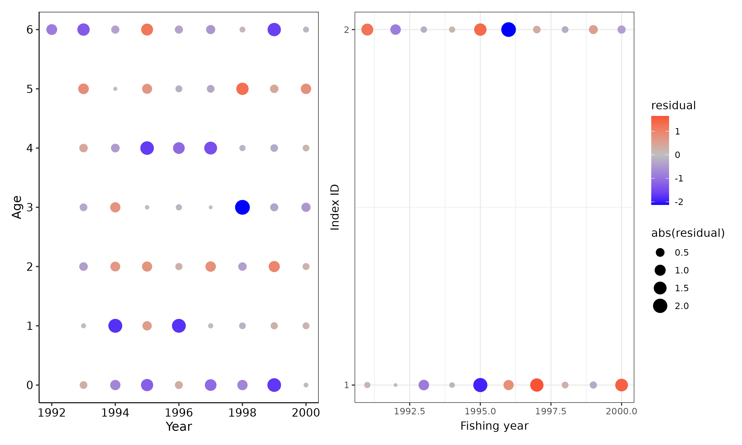

プロファイル尤度

• Cachability qなどを変化させたときの対数尤度を調べて、収束しているか、どの程度尤度が変わるか（不確実性の程度、信頼区間）を調べる

# Catchabilityに対するプロファイル尤度
# 同じ名前のパラメータが複数ある場合は引数\code{which_param}で位置を指定できる
res_profile <- samprofile(res_best, "logQ", which_param=1, param_range=c(8, 11), length=25)

# 縦軸は負の対数尤度
res_profile$obj_tbl[-1,] %>%
  ggplot(aes(x=par, y=obj_value)) + geom_line(linewidth=0.5) +
  geom_point(data=res_profile$obj_tbl[1,],colour="red")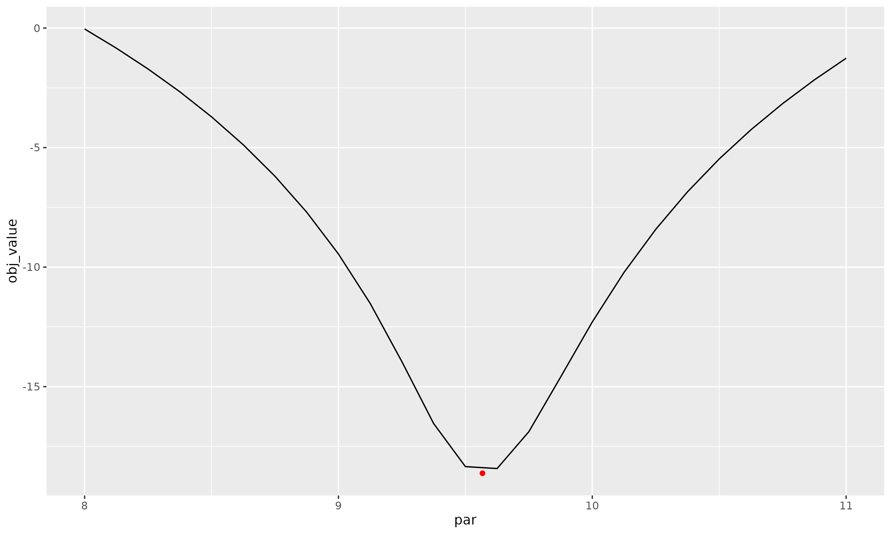

# Mのプロファイル尤度 => 関数がないからこんな感じで手動で
Ms = c(0.1,0.3,0.5,0.7,0.9)
scns = str_c("M:",Ms)
samres_Mlist = map(Ms, function(i) {
  res = res_best
  p0_list = res$par_list
  input = res$input
  input$dat$M[] <- i
  res.c = do.call(sam,input)
  return( res.c )
})

data.frame(
  M = Ms,
  obj_value = sapply(samres_Mlist, function(x) x$opt$objective)
) %>% ggplot(aes(x=M,y=obj_value)) + geom_line() + geom_point()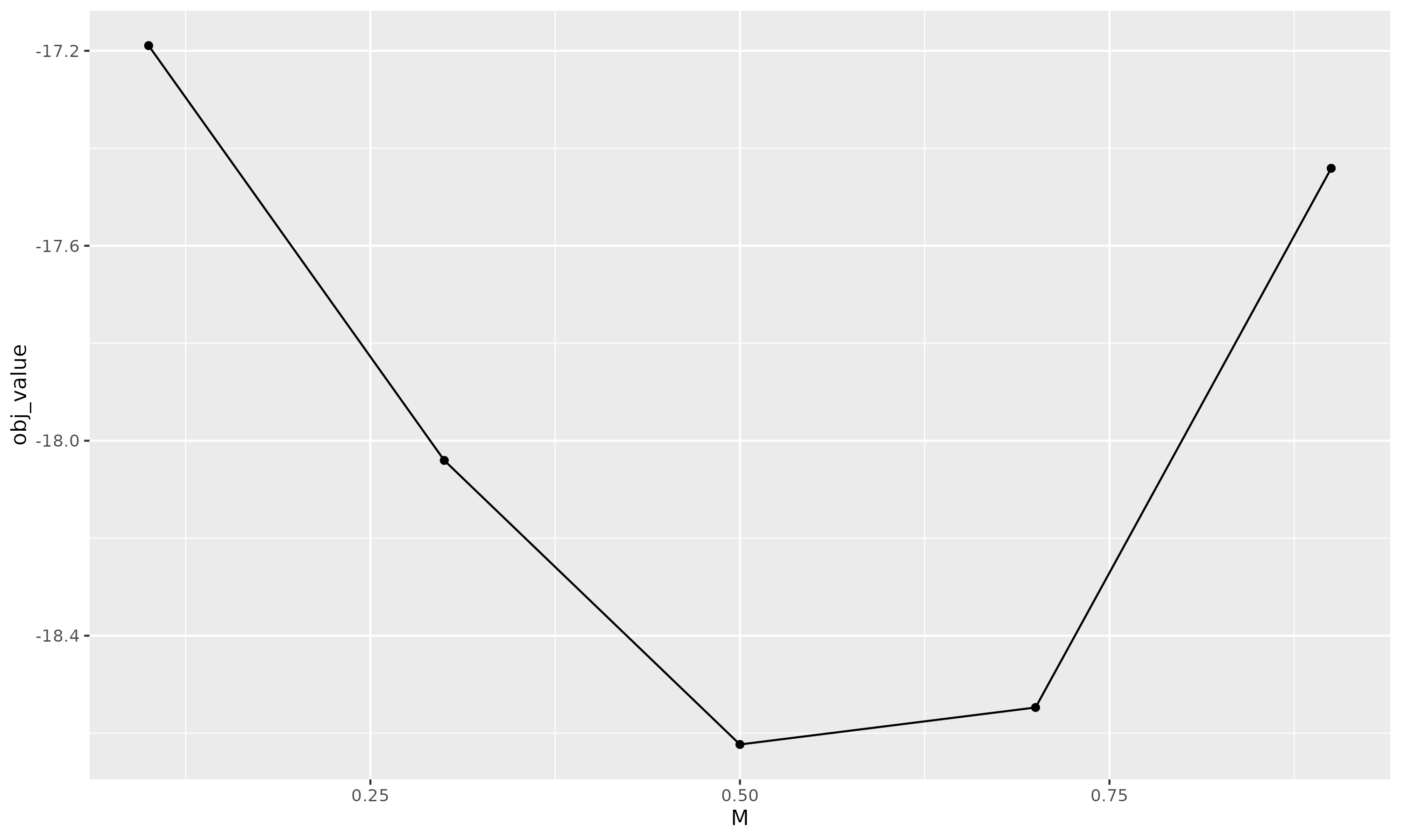

plot_samvpa(samres_Mlist,scenario_name=scns,CI=0.)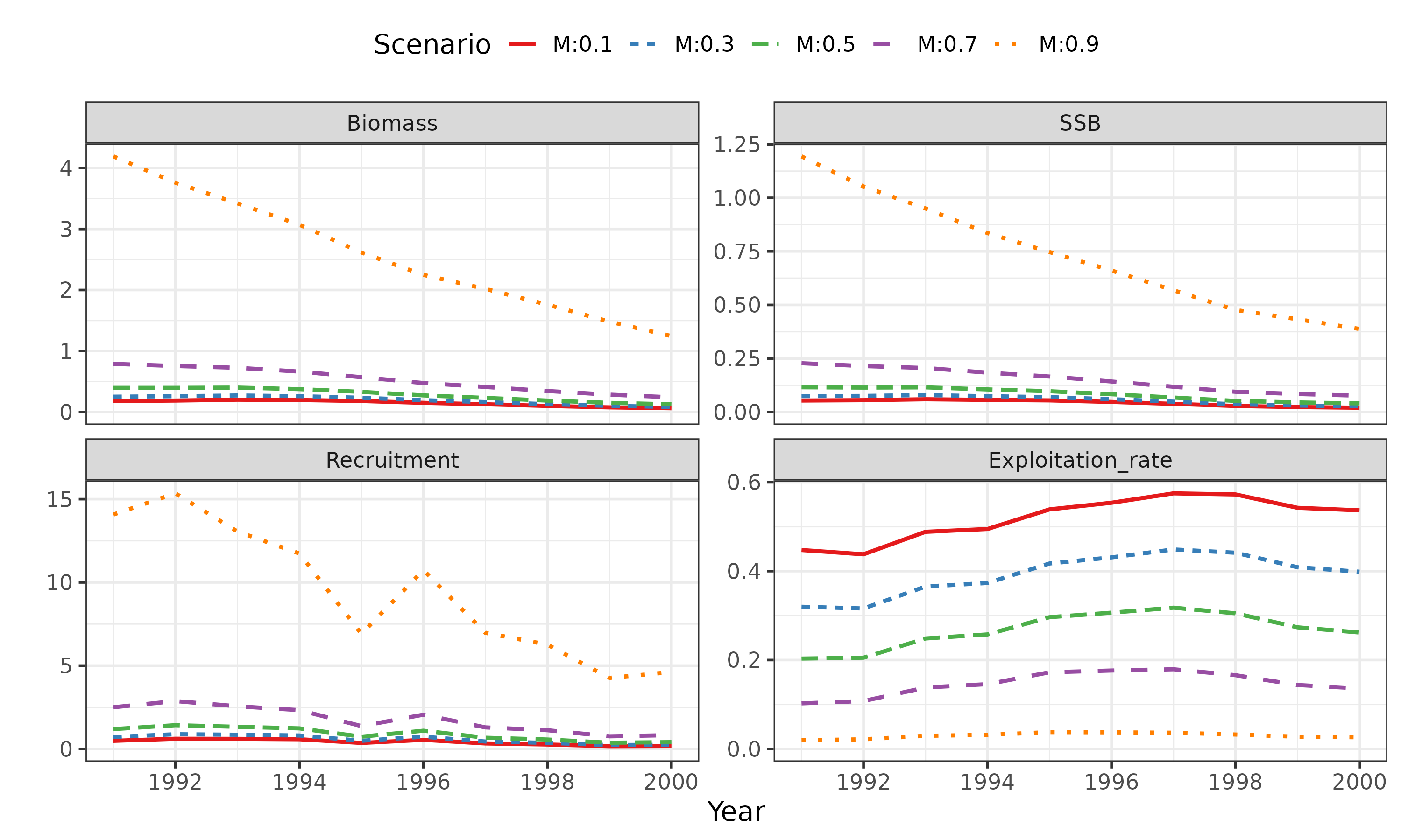

ブートストラップ

• で実行できる
• ノンパラメトリックブートストラップ（）は厳密ではないので、パラメトリックブートストラップを推奨（）
• delta法で求めたCIも図に加える場合は

res_boot <- boo_sam(res_best, n=20,method="p",seed=1) #時間節約のため20回
#> -----1-----
#> -----2-----
#> -----3-----
#> -----4-----
#> -----5-----
#> -----6-----
#> -----7-----
#> -----8-----
#> -----9-----
#> -----10-----
#> -----11-----
#> -----12-----
#> -----13-----
#> -----14-----
#> -----15-----
#> -----16-----
#> -----17-----
#> -----18-----
#> -----19-----
#> -----20-----
(g1 = plot_boosam(res_sam2,res_boot, CI=0.95, draw_deltaCI = TRUE))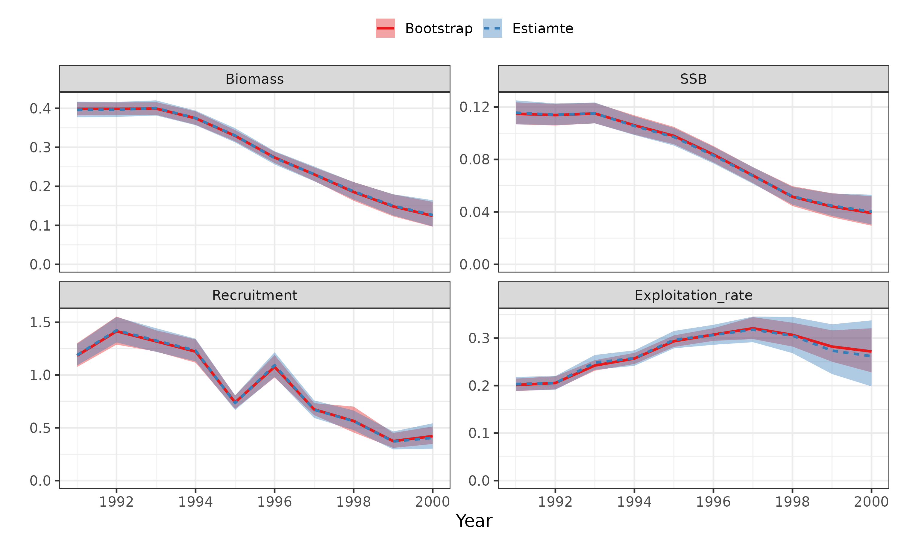

Self-test / cross test

• 真のモデルをVPA or SAMとして、疑似データを生成し、VPA or SAMのモデルを疑似データにフィットさせるというシミュレーションが可能
• 真のモデル (operating model, OM) と推定モデルが同じモデルであればselt-test, 異なればcross-test
• VPA or SAMのestimability (self-test), 異なる仮定に対する推定の頑健性 (cross test) を調べられる

## 真のモデルはSAM
# pseudo dataを生成
pdata_sam <- popsim_vpasam(res_best, n=20)
# self-test (SAMで推定)
# 前述のブートストラップと同じ（はず）
fit_sam2sam <- fit2PSdata(res_best, PSdata=pdata_sam)
metric_sam2sam = sumup_popsim(res_best,fit_sam2sam) #真のモデルの結果を使うこと
# SSBの要約統計量を出力
metric_sam2sam$summary %>% filter(stat=="SSB") %>% knitr::kable()

stat	year	age	RMSE	MAE	RMSRE	MARE	MedBias	MedRelBias	Median	CV	value_true	lower	upper
SSB	1991	NA	4.714890	3.739724	0.0407805	0.0323460	0.6798051	0.0058798	116.29599	0.0402735	115.61619	108.23633	124.31695
SSB	1992	NA	4.470541	3.417776	0.0391776	0.0299517	0.6635134	0.0058147	114.77299	0.0384901	114.10948	108.00884	124.11675
SSB	1993	NA	3.981475	2.961603	0.0345664	0.0257121	-0.7306428	-0.0063433	114.45279	0.0354558	115.18344	108.50679	123.23835
SSB	1994	NA	3.916236	3.049157	0.0371171	0.0288992	-0.5248452	-0.0049744	104.98534	0.0374849	105.51019	99.88823	113.44926
SSB	1995	NA	3.353828	2.650598	0.0345464	0.0273027	-0.7773941	-0.0080076	96.30453	0.0354207	97.08192	91.91651	104.10862
SSB	1996	NA	3.156222	2.498548	0.0379865	0.0300711	0.2791449	0.0033596	83.36722	0.0387767	83.08808	77.38519	88.79782
SSB	1997	NA	3.152909	2.535913	0.0467273	0.0375832	-0.0284438	-0.0004215	67.44623	0.0479250	67.47468	62.47695	73.73288
SSB	1998	NA	3.542636	3.009047	0.0682894	0.0580037	0.2051571	0.0039547	52.08197	0.0683529	51.87681	46.55599	58.09936
SSB	1999	NA	4.224429	3.418742	0.0944754	0.0764570	0.1067732	0.0023879	44.82137	0.0973533	44.71460	38.61181	52.98685
SSB	2000	NA	5.503604	4.265156	0.1368733	0.1060734	-0.5414189	-0.0134650	39.66807	0.1416574	40.20949	32.56410	51.16901

(g_sam2sam <- plot_popsim(res_best,fit_sam2sam))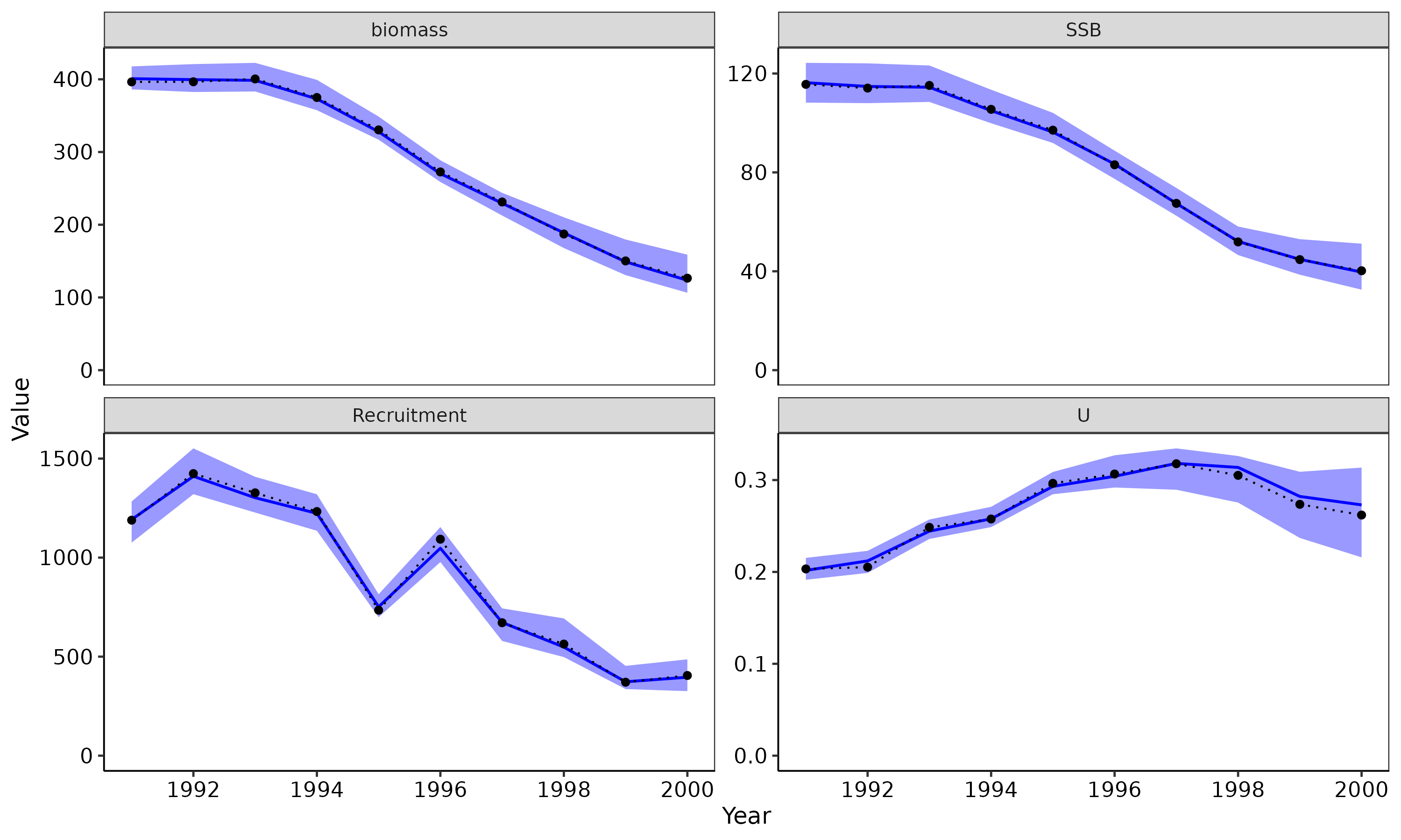

# cross-test (VPAで推定)
# 前述のブートストラップと同じ（はず）
fit_vpa2sam <- fit2PSdata(res_vpa, PSdata=pdata_sam) #ここでは別のモデルを使う
metric_vpa2sam = sumup_popsim(res_best,fit_vpa2sam) #こっちでは真のモデルの結果を使うこと!
# SSBの要約統計量を出力
metric_vpa2sam$summary %>% filter(stat=="SSB") %>% knitr::kable()

stat	year	age	RMSE	MAE	RMSRE	MARE	MedBias	MedRelBias	Median	CV	value_true	lower	upper
SSB	1991	NA	6.471087	5.529497	0.0559704	0.0478263	5.340624	0.0461927	120.95681	0.0408417	115.61619	110.48940	127.03547
SSB	1992	NA	6.344622	5.089540	0.0556012	0.0446023	3.590157	0.0314624	117.69963	0.0395019	114.10948	110.64467	127.82181
SSB	1993	NA	5.992787	4.777344	0.0520282	0.0414760	3.365942	0.0292224	118.54938	0.0371021	115.18344	111.95927	127.80785
SSB	1994	NA	6.375684	4.992017	0.0604272	0.0473131	4.063816	0.0385159	109.57400	0.0443690	105.51019	101.73084	119.76746
SSB	1995	NA	6.128014	4.745004	0.0631221	0.0488763	4.133170	0.0425740	101.21509	0.0426599	97.08192	95.57532	110.62512
SSB	1996	NA	6.237325	4.913610	0.0750688	0.0591374	4.487785	0.0540124	87.57586	0.0562459	83.08808	79.45123	96.92702
SSB	1997	NA	6.307079	4.863802	0.0934733	0.0720834	3.450676	0.0511403	70.92535	0.0742778	67.47468	63.85060	82.26122
SSB	1998	NA	6.901705	5.284913	0.1330403	0.1018743	4.289524	0.0826867	56.16634	0.0997085	51.87681	48.74747	67.64629
SSB	1999	NA	7.090084	4.946232	0.1585631	0.1106178	3.154422	0.0705457	47.86902	0.1342297	44.71460	40.62752	61.98933
SSB	2000	NA	8.516743	6.248140	0.2118093	0.1553897	1.960584	0.0487592	42.17008	0.1892163	40.20949	33.98896	60.50028

(g_vpa2sam <- plot_popsim(res_best,fit_vpa2sam))

# SAMの結果（res_best）の代わりに、VPAの結果をoperating model (真のモデル) として入れ替えて、VPAデータに対するself-test / cross-testもできます

将来予測

• 資源量推定の不確実性をどこまで考慮するか？
• 再生産関係は外部で推定しても良いのかも（難しいことはしなくてもよいようにもしておく）